UPDATED 08/30/2020 – O. angasi Gonad Image Segmentation Protocol

This protocol goes over the image segmentation process for O. angasi histology images conducted in the first half year of 2020. This process uses two scripts:

create_ density_plots.py
- Creates sperm and egg composite images and also creates the color density plots to analyze the range of values for color spaces used
gonad_ image_segmentation.py
- Segments histology images and creates csv file containing segmentation info about each image

Preliminary items needed:

A directory containing histology images to be analyzed (will be called histology directory from here on out)
- histology images should be labeled numerically
A directory to place sperm & egg composite images and color density plots in (will be called color directory from here on out)

create_ density_plots.py

(This script is heavily based off of the article Color Spaces in OpenCV (C++/Python))

Place the create_ density_plots.py script into the color directory
Use a random number generator to generate at least 10 random numbers from a range of values consistent with the number of histology images present in the histology directory
- From each of the 10 numbers generated, open the corresponding histology images:
  - Take a standardized number of screenshots per each image of the egg and/or sperm present in the image
  - Save the screenshots into the color directory
Open the file create_ density_plots.py
Write filenames of all egg screenshots taken in the “egg” list (see line 8)
Write filenames of all sperm screenshots taken in the “sperm” list (see line 14)
Write the filename for the composite image that will be created from the egg images on the “image_ name_egg” line (see line 19)
Write the filename for the composite image that will be created from the sperm images on the “image_ name_sperm” line (see line 21)
In order to create the composite images, each screenshot used to create the composite needs to have the same dimensions. Thus, to standardize the dimensions of:
- egg screenshots: write standardized length and height desired on line 30
- sperm screenshots: write standardized length and height desired on line 34
To create the color density plots to analyze the composite image desired, write the variable name of the composite image in line 24 (e.g., if you want to analyze the egg composite image, write “image_ name_egg” for the “what to read” variable)
To choose the color space to analyze the composite image in, use the function cv2.COLOR in line 49 (e.g., to analyze the image in the YCrCb color space, use the function “cv2.COLOR_BGR2YCrCb)
Lines 51 - 66 of the script essentially separate the channels of the color space in order to visualize each channel on an axis of the color density plots; you don’t necessarily have to change the variable names to match the color space in order for this to work, but it may be helpful just to help keep track (e.g, if you want to analyze the YCrCb version, you can use “Y” instead of “B” for lines 51 and 62, use “CR” instead of “G” for lines 52 and 63, use “CB” instead of “R” for lines 54 and 64,use “y” instead of “b” for lines 56 and 57, use “cr” instead of “g” for lines 58 and 59, and use “cb” instead of “r” for lines 60 and 61). But, if you do this, just make sure to standardize it with the variables in line 66, since this is the line where you choose which channels are going to be shown on the density plot
To choose which channels to display on the color density plot, write down the associated channel variable on line 66 (e.g., if you want to view the color plot with the color channels B and G of the color space BGR, with B on the x-axis and G on the y-axis, you would write “plt.hist2d(B, G, bins = nbins, norm = LogNorm())” for line 66)
To label x-axis of color plot with corresponding color channel, write name of channel on line 68 (e.g., if x-axis shows “B” color channel, write “plt.xlabel(‘B’)” for line 68)
To label y-axis of color plot with corresponding color channel, write name of channel on line 69
Write path to directory to save color density plot created on line 72
Run the script
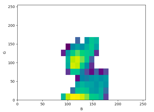
Once the plot is created, visually analyze the plot to see the range of color values that are present in the composite image for the channels listed
- E.g., for the density plot below, the range of values for the channel “B” are from a minimum of 80 to a maximum of 160 and the range of values for the channel “G” are from a minimum of 0 to a maximum of 175
Repeat steps 10 thru 16 for all 4 color spaces (BGR, HSV, Lab, YCrCb) in order to create color density plots and obtain the minimum and maximum color values for each color channel of all 4 color spaces; change the “what to read” variable on line 24 to repeat this process for both the egg composite image and the sperm composite image
When the minimum and maximum values for all color channels of a color space are found, save them in a list-like format; for both the minimum and the maximum values, write the list as [first channel, second channel, third channel]
- e.g, for the BGR color space, if the range of values for B is from 80 - 160, G is from 0 - 175, and R is from 140 - 250, then the minimum channel list would be [80, 0, 140] and the maximum value list would be [160, 175, 250]
  - Repeat this for all 4 color channels

gonad_ image_segmentation.py

Save the file gonad_ image_segmentation.py in the histology directory
Open the file gonad_ image_segmentation.py
Write path to histology directory in lines 7 and 15
Write the filename of the output csv that will contain the segmentation data for all histology images analyzed on line 10
Depending on image type and format, write corresponding image type on line 16 (e.g., if image type is .tif, then write “filename.endswith(‘.tif’)); for these specific images, only looked at the images with 10x magnification, which is why there is “filename[19] == “1”” added to this line – remove this if this does not apply to the specific kinds of images that you are analyzing
Using the minimum and maximum values for each of the 4 color spaces found in step 19 of the create_ density_plots.py script, write the values down in these lines:
- For egg segmentation:
  - minimum values for BGR: line 37
  - maximum values for BGR: line 38
  - minimum values for HSV: line 56
  - maximum values for HSV: line 57
  - minimum values for YCrCb: line 76
  - maximum values for YCrCb: line 77
  - minimum values for Lab: line 96
  - maximum values for Lab: line 97
- For sperm segmentation:
  - minimum values for BGR: line 119
  - maximum values for BGR: line 120
  - minimum values for HSV: line 138
  - maximum values for HSV: line 139
  - minimum values for YCrCb: line 158
  - maximum values for YCrCb: line 159
  - minimum values for Lab: line 178
  - maximum values for Lab: line 179
Run the script
- Segmented images and csv file will appear in histology directory

Post-Image Segmentation - Organizing files in Google Drive

I used Google Drive in order to organize the segmentation information and segmented images in one place:

Place original and segmented histology images in a folder in Google Drive
Create a Google sheet
Copy and paste the summarized segmentation information created in the csv file output from the gonad_ image_segmentation.py script into the Google sheet
- Make sure that the information is in numerical order according to filename (this will be helpful when organizing the associated image links)
Once the information is pasted in, create 5 columns with headers for the original file image links, the BGR segmentation image links, the HSV segmentation image links, the Lab segmentation image links, and the YCrCb segmentation image links
In the spreadsheet, click on an empty column that is not any of the columns previously mentioned
Go to the “Tools” tab in the spreadsheet and click on “Script editor”
In the newly opened tab, write in this script (got this script online, but it seems this script appears in a lot of different places, so here’s just one link for reference: Get share link of multiple files in Google Drive to put in spreadsheet) in order to create a list of image links that are associated to each image in the folder where you saved all of the histology images:
- For a folder with the url, https://drive.google.com/drive/folders/id, write:
function myFunction(){
```
 var ss=SpreadsheetApp.getActiveSpreadsheet()
 var s=ss.getActiveSheet();
 var c=s.getActiveCell();
 var fldr=DriveApp.getFolderById("id");
 var files=fldr.getFiles();
 var names=[],f,str;
 while (files.hasNext()) {
     f=files.next();
     str='=hyperlink("' + f.getUrl() + '","' + f.getName() + '")';
     names.push([str]);
     }
 s.getRange(c.getRow(),c.getColumn(),names.length).setFormulas(names);  }
```
Click on the Play button to run the script
Once the script runs, a list of image links should appear in the column that was clicked in step 5
- The list should be in numerical order, with an original image appearing every 5 lines, a BGR image appearing every 5 lines, a HSV image appearing every 5 lines, etc…
In order to separate the image links into their associated columns, click under the column name you would like to add the image links to, and copy and paste this line down as far as needed (line based off of this forum): {
- For a list of image links appearing in column ZZZ, in the order
  - A
  - B
  - C
  - D
  - E
- If you would all image links associated with A to be in the column clicked, write:
```
  =INDEX($ZZZ:$ZZZ,ROW(A1)*5-5+COLUMN(A1))
```
- If you would all image links associated with B to be in the column clicked, write:
```
  =INDEX($ZZZ:$ZZZ,ROW(B1)*5-5+COLUMN(B1))
```
- If you would all image links associated with C to be in the column clicked, write:
```
  =INDEX($ZZZ:$ZZZ,ROW(C1)*5-5+COLUMN(C1))
```
- Etc, etc…
Using all of these steps, all segmentation information and image links to the associated images should be organized onto one sheet for easy analyzation!